Many statistical terms are daunting and can quickly become confusing. Even scholars themselves do not agree on what some mean. Try asking what a p-value is at a conference or, if you want to see academics practice kung-fu, ask them whether one should use fixed or random effects (safety not guaranteed). Many concepts sound alike and statistical learners end up feeling like reading a Russian novel: who is Alexandra Petrovna again? And what is her relation to Peter Alexandrovitch? Sometimes, it is even hard to distinguish statistical concepts from expletives used by Captain Haddock. Being a non-native speaker compounds these difficulties.

I have not yet come across a statistical book with an accessible glossary. So I hope this simple dictionary (slowly updated, work-in-progress!) will help you (and me) to survive the life statistical. Let me know where I can improve it!

Also, caveat lector!

Alphabetically

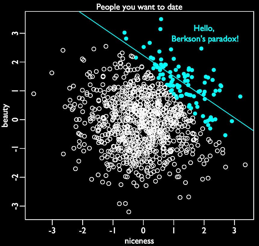
• Berkson’s paradox: named after Berkson (1946), it can be called the selection-distortion effect or conditioning on a collider: here, spurrious correlation is caused by a common effect. The selection bias, or the act of selecting, creates a correlation between unassociated variables. Imagine there are 1 000 persons you could date. Among them, beauty and niceness are randomly distributed and uncorrelated. Some are both, some are neither, and some are either. But you rank the 10% you want to date, weighting beauty and niceness equally. Your strong selection induces a (strong, negative) correlation between the unrelated beauty and niceness. How is that magic possible? Because the people you selected are either beautiful and/or nice, and because you avoid dating people who are neither nice nor beautiful. This selection creates this distortion. If you don’t believe me, check the simulation below!
  • See also: collider, selection

1
2
3
4
5
6
7
8
9
10
11
12
13
14
15

set.seed(2021)
candidates <- 1000 # number of people you want to date
select <- 0.1 # proportion to select
# uncorrelated beautiness and niceness 
beauty <- rnorm(candidates)
niceness <- rnorm(candidates)
# select top 10% of combined scores
date <- beauty + niceness # total score
nothot <- quantile( date , 1-select ) # top 10% threshold 
selected <- ifelse( date >= nothot , TRUE , FALSE )
# let's plot it
plot(beauty ~ niceness, 
     pch=ifelse( date >= nothot , 16 , 1 ) ,
     col=ifelse( date >= nothot , "red" , "black" ))
abline(lm(beauty[selected] ~ niceness[selected]), col="red")

• Bootstrapping: or how statistics proved that the expression “pull oneself up by one’s bootstraps” can actually make sense and that Baron Munchausen was a statistical precursor. Bootstrap means resampling randomly your dataset many times (thus creating many samples) to calculate an estimate, its standard errors and confidence intervals. Each of these new samples has it own characteristics (mean, median etc): if you take all these samples, you can have a distribution of these characteristics (the sampling distribution). Contrast this to standard hypothesis testing, which requires test statistics and assumptions.
  • See also: jackknife, cross validation, information criteria, hypothesis testing
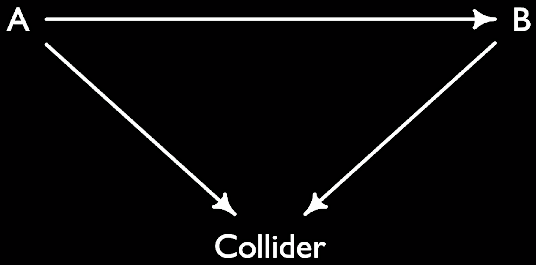
• Collider: common effect of two causes. In DAGs, colliders are where two arrows collide. If you condition on a collider, a spurrious association arises between two causes even though there is no causal relation between them. This is due to the fact that information circulates from one cause to the effect to the second cause. It is rarely a good idea to condition on colliders in a regression, as Berkson’s paradox shows!
  • See also: DAG, selection bias, Berkson’s paradox, confounder, mediator

1
2
3
4

library(dagitty)
collider <- dagitty( "dag{ A -> Collider; B -> Collider }" ) 
coordinates(collider) <- list( x=c(A=0,Collider=1,B=2) , y=c(A=0,Collider=1,B=0) ) 
plot(collider)

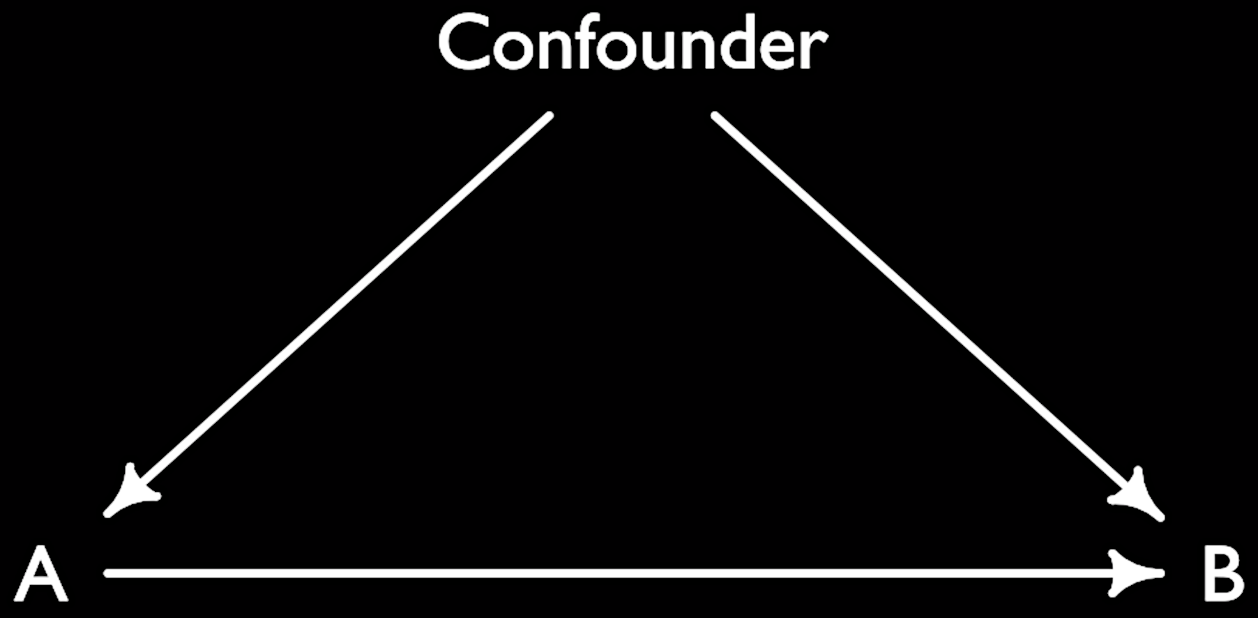
• Confounder: Variable influencing both our treatment/exposure/pet variable and our outcome. The confounder is thus a common cause and should be conditioned on. It can be also called omitted variable bias.
  • See also: Berkson’s paradox, collider, DAG, mediator, selection bias

1
2
3
4
5

library(dagitty)
confounder <- dagitty( "dag{ A -> B; A <- Confounder; B <- Confounder }" ) 
coordinates(confounder) <- list( x=c(A=0,Confounder=1,B=2) , 
		y=c(A=1,Confounder=0,B=1) ) 
plot(confounder)

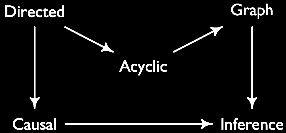
• DAG (directed acyclic graph): DAGs help to describe relationships between variables. Directed, because the graph indicates the direction of causality between variables. Acyclic, because the causality goes not go back. Graph, because variables are nodes and ties are their relationships. DAGs represent our assumptions about the model that we want to estimate.
  • See also: Judea Pearl, confounder, collider, selection bias, Berkson’s paradox, mediator

1
2
3
4
5
6

library(dagitty)
DAG <- dagitty( "dag{ Directed -> Acyclic; Acyclic -> Graph; Graph -> Inference; 
		Directed -> Causal; Causal -> Inference }" ) 
coordinates(DAG) <- list(x=c(Directed=0,Acyclic=.5,Graph=1,Causal=0,Inference=1),
		y=c(Directed=0,Acyclic=.5,Graph=0,Causal=1,Inference=1)) 
plot(DAG)

• Dendogram: a dendrogram is a hierarchical tree that predicts the possible community partitions. Used mostly in cluster analysis. In network analysis can be used to identify communities.

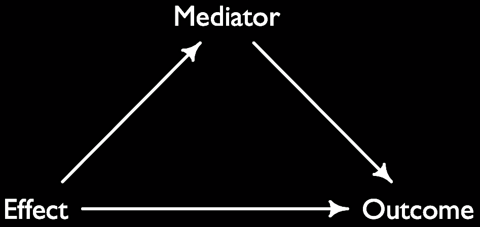
• Effect: the effect of a treatment on an outcome can take several forms: it can be total, direct and indirect. The total effect is the entire effect of a treatment (independent) variable on the outcome. The direct effect is the effect that is not mediated by an intervening/mediator variable (there is nothing on the path between treatment and outcome). The indirect effect is when a treatment (independent) variable impacts an outcome (dependent) variable one or more intervening/mediator variables.
  • See also: mediation, intervening variable, table 2 fallacy

1
2
3
4
5
6

library(dagitty)
Effect <- dagitty( "dag{ Effect -> Outcome; Effect -> Mediator; 
						 Mediator -> Outcome }" ) 
coordinates(Effect) <- list( x=c(Effect=0, Outcome=2, Mediator=1), 
				y=c(Effect=1, Outcome=1, Mediator=0) ) 
plot(Effect)

• Kurtosis: neither an insult nor a planet. Rather, kurtosis quantifies how fat the tails of a distribution are. It’s also called the fourth moment of a distribution.

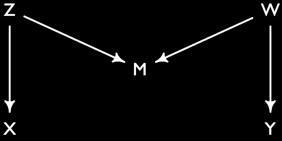
• M-Bias: Controlling for a collider that is a pre-treatment variable. Here Z is a (latent) cause of X, the treatment, and W the (latent) cause of Y, the outcome. Z and W are uncorrelated in the simple version of the M-bias.

1
2
3
4

library(dagitty)
Mbias <- dagitty( " dag{ X <- Z ; Z -> M ; W -> M ; W -> Y }")
coordinates(Mbias) <- list(x=c(X=0, Z=0, M=1, W=2, Y=2), y=c(X=2, Z=0, M=1, W=0, Y=2))
plot(Mbias)

• Mediator/Mediation: A mediator is a variable on the causal path between a treatment/exposure A and an outcome B.
  • See also: effects (total, direct and indirect)

1
2
3
4

library(dagitty)
mediation <- dagitty( "dag{ A -> Mediator -> B}" ) 
coordinates(mediation) <- list( x=c(A=0,Mediator=.5,B=1) , y=c(A=1,Mediator=1,B=1) ) 
plot(mediation)

• Multilevel or hierarchical models: models whose parameters vary by groups/clusters.
  • See also: cross-classified model, fixed effects, hyper priors, pooling, random effects, regularization, shrinkage, varying intercepts, varying effects

• Prior: Simply put, a prior is the plausibility of your hypothesis in the absence of evidence.

• Probability: Does probability exist? If yes, what is it? It’s surprising to learn that there is no agreement on this. Some people like Bruno de Finetti claimed that probability does not exist - at least not objectively. It’s in the eye of the beholder: many people have different probabilities of an event depending on their state of knowledge. Others defined probability base on notions such as a set of events (Kolmogorov), a long run frequency (Venn), or based on all possible outcomes of an experiment (Gosset).

• Regularization: Sometimes, our stats models learn too much from the data at hand: they get overhyped and think that some of the noise (random stuff) is actually signal (the real stuff). This happens especially when we have lots of parameters (sometimes more than data points). So we would like something that helps us avoid this problem of “overfitting”. One solution in Bayesian stats is to have “regularizing” priors, i.e. which tell our model to take it easy and shrink coefficients towards zero. Another solutions is to use lasso or ridge regression to reduce coefficient variance. You can also think of regularization as a penalty on the parameters. The paradox is that regularization yields better predictions by making the model worse at fitting the sample.
  • See also: underfitting, overfitting, lasso, ridge, shrinkage, multilevel models

• Skewness: skewness measures how symmetric a distribution is. It is also called the third moment of a distribution.

• Table 2 fallacy: When you present regression results in a table (typically the second table after the descriptive statistics of your data) and interpret all coefficients from your pet variable (the “exposure”) to the confounders as if they were all the same causal total effects. But this is not necessarily the case: depending on your DAG, your coefficients can represent for instance total or direct effects. Also, while the effect of your exposure may be unconfounded, it does not imply that the effect of the confounders is also unconfounded (e.g. because of unmeasured confounders). Well, that was a mouthful! Welcome to stats!

  • See also: effect, DAG
  • Source: Westreich and Greenland (2013)

Acknowledgments

Thanks to Alex Moise, Aki Suzuki and Joe Ganderson!